



Luigi Piva, CQF — Quanthedge AI (research arm of AlgosWorks AI Ltd)
All code in this article is runnable as-is. The example track record is synthetic and fully specified, so every number is reproducible;
Search for “Monte Carlo simulation trading strategy” and you will find, with remarkable consistency, the same recipe: take the list of your backtest trades, shuffle their order a few thousand times, recompute the equity curve each time, and read off a distribution of drawdowns. This is presented as “Monte Carlo analysis” of your system, and it is supposed to tell you what risk to expect going forward.
It is not Monte Carlo. It is not even a well-specified bootstrap. It is a permutation of your sample, and for the one question it is usually asked to answer, the depth of future drawdowns, it is biased in the most dangerous direction: it makes your strategy look “safer” than the data says it is.
This article does three things. It defines precisely what the bootstrap is and what Monte Carlo is, two different tools that answer two different questions. It shows, with code and numbers, how the popular shuffle systematically thins the drawdown tail whenever returns exhibit the serial structure that real strategy returns always exhibit. And it ends with an operational taxonomy: which question you are asking, and which procedure is entitled to answer it.
The Canonical Error
Here is the forum recipe, stated honestly for what it is:
1. Take the sequence of realised P&L (trades or daily returns).
2. Randomly permute the sequence B times.
3. For each permutation, rebuild the equity curve and record max drawdown, time under water, etc.
4. Report percentiles of that distribution as “what could have happened”.
Two assumptions are buried in step 2, and both are false for trading strategies.
First: exchangeability: A permutation treats every ordering of your P&L as equally likely, which is only true if the observations are independent and identically distributed. Strategy returns are not i.i.d. Volatility clusters, turbulent weeks follow turbulent weeks and most systematic strategies have some serial dependence in returns themselves: trend systems bleed in small correlated losses and win in correlated runs; mean-reversion systems do the opposite. The regime structure of markets induces regime structure in your P&L.
Second: the sample is the population: Shuffling never produces a return that did not occur in your backtest. It cannot generate a volatility level you have not seen, a correlation breakdown you have not lived through, or a losing streak longer than combinatorics of your own history allows. It recycles the past in a different order; it creates no new information about the world.
Now, why does this specifically understate drawdown risk? Because maximum drawdown is a functional of the path, and the path property that produces deep drawdowns is precisely the clustering of bad outcomes. Permutation destroys clustering by construction: it takes your correlated losing streaks, breaks them apart, and sprinkles the pieces uniformly through time. The resampled equity curves are smoother than any curve your strategy could actually produce. The distribution of simulated drawdowns is pulled toward zero, and its bad tail, the only part you care about, is the most distorted of all.
Let’s quantify it.
A reproducible testbed
I need a return series with the two features that matter, volatility clustering and mild serial dependence and I want it fully specified so you can rerun everything. A two-state Markov regime process with a light AR(1) overlay does the job; it is a caricature of a real futures strategy track record, but a caricature with the right anatomy. (When you rerun this on your own strategy, delete this block and load your returns.)
“`python
import numpy as np
rng = np.random.default_rng(42)
n = 2520 # ~10 years of daily returns
P = np.array([[0.99, 0.01],
[0.04, 0.96]]) # calm <-> turbulent transitions
mu = np.array([ 0.0008, -0.0004]) # daily drift by regime
sig = np.array([ 0.006 , 0.016 ]) # daily vol by regime
states = np.zeros(n, dtype=int)
for t in range(1, n):
states[t] = rng.choice(2, p=P[states[t-1]])
eps = rng.normal(mu[states], sig[states])
r = np.empty(n)
r[0] = eps[0]
for t in range(1, n):
r[t] = 0.08 * r[t-1] + eps[t] # mild serial dependence
def sharpe(x):
return x.mean() / x.std(ddof=1) * np.sqrt(252)
def max_drawdown(x):
w = np.cumprod(1.0 + x)
return (w / np.maximum.accumulate(w) – 1.0).min()
“`
The realized history: Sharpe 0.76, maximum drawdown −41.5%**, first-order autocorrelation of 0.12 in returns and 0.16 in squared returns. Nothing exotic, these are unremarkable numbers for a mid-frequency futures programme, and exactly the kind of dependence structure the shuffle assumes away.
What the Bootstrap actually is
The bootstrap (Efron, 1979) answers a specific question: given that I observed this sample, how uncertain is a statistic computed from it? You resample from the empirical distribution — with replacement — recompute the statistic each time, and use the resulting spread as an estimate of the sampling distribution. It is a device for putting confidence intervals around your Sharpe ratio, your CAGR, your drawdown, without assuming normality.
The textbook version resamples individual observations, and that is where the i.i.d. assumption sneaks back in. Resampling single days destroys serial structure just as thoroughly as shuffling does. For dependent data you need the block family:
-Moving block bootstrap (Künsch, 1989): resample contiguous blocks of fixed length.
– Stationary bootstrap(Politis–Romano, 1994): blocks of *geometrically distributed* random length, which keeps the resampled series stationary and removes the artificial seams of fixed blocks.
– Block length is a bandwidth parameter; Politis–White (2004) give an automatic selection rule. In practice, for daily strategy returns, mean blocks of 10–40 days bracket the answer, and you should report sensitivity rather than a single sacred number.
Here is a compact, vectorised stationary bootstrap:
“`python
def sb_indices(n, mean_block, rng):
“””Politis-Romano stationary bootstrap index sequence.”””
p = 1.0 / mean_block
restarts = rng.random(n) < p # geometric block ends
restarts[0] = True
block_id = np.cumsum(restarts) – 1
pos = np.arange(n)
offsets = pos – pos[restarts][block_id]
starts = rng.integers(0, n, restarts.sum())
return (starts[block_id] + offsets) % n # circular wrap
def stationary_bootstrap(x, stat, B=5000, mean_block=20, rng=rng):
n = len(x)
return np.array([stat(x[sb_indices(n, mean_block, rng)])
for _ in range(B)])
def shuffle_dist(x, stat, B=5000, rng=rng): # the forum recipe
return np.array([stat(rng.permutation(x)) for _ in range(B)])
def iid_bootstrap(x, stat, B=5000, rng=rng): # textbook bootstrap
n = len(x)
return np.array([stat(x[rng.integers(0, n, n)]) for _ in range(B)])
“`
What can a (correct) bootstrap tell you? The uncertainty of statistics of the history you actually had. What can it not tell you? Anything about states of the world absent from your sample. If your ten years contain no 2008, no block resampling will manufacture one. Keep that limitation in mind; it is the door through which real Monte Carlo enters later.
The Numbers
Tab.1 Running all three
procedures on the same series, B = 5,000 each:
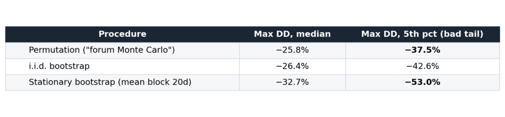
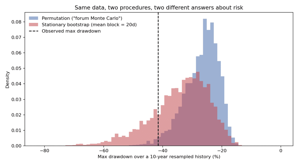
Read the first row carefully. The strategy’s actually realised drawdown was −41.5%. The shuffle-based distribution puts its 5th percentile, the “bad scenario” a practitioner would provision against at −37.5%. The permutation analysis declares the drawdown that already happened to be worse than its own 1-in-20 adverse scenario. If you sized capital, set investor expectations, or placed a system kill-switch using that distribution, reality has already violated your risk model, using no data other than the data you fed it.
The stationary bootstrap, which preserves the local dependence structure, tells a different story: median resampled drawdown −32.7%, bad tail at −53.0%. The realized −41.5% sits comfortably inside the body of this distribution, as it should, the procedure is consistent with the evidence that produced it.
The i.i.d. bootstrap lands in between, and it is worth understanding why it looks less catastrophic than the shuffle here: resampling with replacement occasionally draws the same turbulent days multiple times, partially reconstructing bad clusters by luck. It is still wrong, it is wrong with noise instead of wrong with a smile and on the Sharpe ratio the damage shows up directly: the i.i.d. 95% confidence interval is [0.15, 1.36], the stationary-bootstrap interval is [0.03, 1.53].
Positive serial dependence inflates the standard error of the Sharpe ratio (this is Lo’s 2002 point in resampling form), so the i.i.d. interval is too narrow: it reports more certainty about your edge than the data contains. The dependence-aware interval brushes zero. That is not a pleasant thing to learn about a Sharpe-0.76 track record, but it is the true state of the evidence — and knowing it is the entire purpose of the exercise.
Figure 1: overlaid histograms of max-drawdown distributions, permutation vs stationary bootstrap, with the observed drawdown marked. The permutation histogram visibly cannot reach the left tail the block bootstrap occupies.
What Monte Carlo Actually is
Monte Carlo simulation is a different animal with a different licence. You specify a data-generating process, a probabilistic model of returns, draw synthetic histories from it, run your strategy (or just your P&L functional) over each, and study the outcomes. The defining feature is the model. The bootstrap resamples the world you saw; Monte Carlo generates worlds from a hypothesis.
That is its power and its tax, in one sentence: Monte Carlo can answer counterfactual questions: what if volatility runs 50% hotter for a decade? what if the vol-of-vol doubles? what happens to my drawdown profile under fatter tails? and every answer is conditional on the model being an adequate description of markets. You have exchanged sampling error for model risk. Neither is free; the sin is not knowing which one you are paying.
A minimal honest specimen — fit a GARCH(1,1) with Student-t innovations and an AR(1) mean to the same series, then simulate:
“`python
from arch import arch_model
am = arch_model(100 * r, mean=”AR”, lags=1,
vol=”GARCH”, p=1, q=1, dist=”t”)
res = am.fit(disp=”off”)
M, dd_mc = 2000, np.empty(2000)
for i in range(M):
sim = am.simulate(res.params, nobs=n)
dd_mc[i] = max_drawdown(sim[“data”].values / 100.0)
# counterfactual: raise unconditional volatility ~50%
stress = res.params.copy()
stress[“omega”] *= 1.5**2
“`
Fitted at the base parameters, the GARCH Monte Carlo gives a drawdown bad tail (5th percentile) of −46.1% in the same territory as the stationary bootstrap, which is reassuring: two dependence-aware procedures, one nonparametric and one parametric, agree about this history. But now ask the question the bootstrap *cannot* answer: under the 1.5× volatility counterfactual, the 5th-percentile drawdown moves to −66.8%. No amount of resampling of the observed sample could have produced that number, because that world is not in the sample. This is the legitimate province of Monte Carlo: exploring specified hypotheticals, while stating plainly that −66.8% is a fact about the model, not (yet) a fact about markets.
Operational Taxonomy
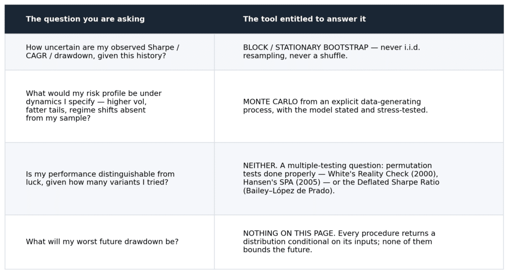
Everything above compresses into four question–answer pairs. This is the part to pin above the desk.
“How uncertain are my observed Sharpe / CAGR / drawdown, given this history?” → Block / stationary bootstrap. Never i.i.d. resampling, never a shuffle.
“What would my risk profile be under dynamics I specify — higher vol, fatter tails, regime shifts absent from my sample?” → Monte Carlo from an explicit DGP, with the model stated and stress-tested.
“Is my strategy’s performance distinguishable from luck, given how many variants I tried?” → Neither. This is a multiple-testing question: permutation tests done properly — White’s Reality Check (2000), Hansen’s SPA (2005) — or the Deflated Sharpe Ratio of Bailey–López de Prado.
“What will my worst future drawdown be?” → Nothing on this page. Any procedure returns a distribution conditional on its inputs; none of them bounds the future.
Two remarks on that third row, because it is where the terminology gets genuinely confusing. There is a valid use of permutation in strategy evaluation — as a null-hypothesis device: permute the signal against the returns (not the P&L against time) to ask whether the alignment of your entries with subsequent moves beats chance. That is a hypothesis test, it is well-posed, and it shares nothing but the word “shuffle” with the forum drawdown recipe. The data-snooping question — you tested 400 parameter sets and are showing me the best one — deserves its own article, and will get one: it is the Bailey–López de Prado programme, and it composes with everything here (you can, and should, block-bootstrap within an SPA test).
What I actually run
For completeness, the validation stack this implies for a mid-frequency futures strategy, in the order the questions arise:
- Stationary bootstrap on daily P&L (mean block 10–40d, sensitivity reported): confidence intervals on Sharpe and drawdown. If the Sharpe CI contains zero, stop here; nothing downstream can rescue it.
- Multiple-testing correction across every variant that was evaluated, not every variant that survived: DSR / SPA.
- Parametric Monte Carlo (GARCH-class or regime-switching DGP) for counterfactual stress: vol scaling, persistence shocks, tail thickening. Outputs are labelled as model-conditional and used for capital buffers, not for performance claims.
- The realised drawdown is always plotted against the resampled distribution. If your procedure calls the past a tail event, the procedure is wrong — fix it before it prices the future.
The shuffle recipe survives online because it is easy, it produces official-looking histograms, and it flatters the strategy. Two of those three properties are also true of the stationary bootstrap — it is fifteen lines of NumPy — and the third one is precisely what honest validation is designed to take away from you.
Reproducibility: NumPy default_rng(42), n = 2520, B = 5000 resamples per procedure, M = 2000 Monte Carlo paths; GARCH estimated with the arch package. Full script available on request — or subscribe to the Market Regime Note, where the code ships with every issue.
References. Efron (1979), Bootstrap methods: another look at the jackknife. Künsch (1989), The jackknife and the bootstrap for general stationary observations. Politis & Romano (1994), The stationary bootstrap. Politis & White (2004), Automatic block-length selection for the dependent bootstrap. Lo (2002), The statistics of Sharpe ratios. White (2000), A Reality Check for data snooping. Hansen (2005), A test for superior predictive ability. Bailey & López de Prado (2014), The Deflated Sharpe Ratio.
Get the monthly Market Regime Note
Regimes, volatility and correlations across major futures markets — with the code behind the charts. Free.
Subscribe →